I mentioned in my first blog post here that I had started to take a data science immersive course at General Assembly, and I figured now would be a good time to cover a little bit of what I had been doing within it. Within the course, as we gradually covered some of the tools to be successful data scientists, we had a number of projects along the way. The project I most enjoyed (so far) was a one-day hackathon of sorts.
We were tasked in groups of three to choose from several Kaggle competitions and have at it. Of the available topics, some were regression, some were classification, some were NLP, and some were image classification. We were told a little after 09:00 on a Monday what was going on and told we would reconvene around 16:00 and go over our results.
09:00:
We start class, and are notified our fourth project was that day. We had turned in our third project before the weekend, and if I had paid more attention to the updated syllabus, I might not have been so blindsided.
09:30:
Having the formalities out of the way and are now in groups. My group spent about the next half hour going through the prompts and tried to decide which problem we would like to tackle. Of all the ones provided, for some reason the challenge on animal shelter outcomes in Austin, TX stood out to us. For a classification problem, it was interesting in more ways than one. To begin with, who doesn’t like the story of dogs and cats finding a home? Now finding a home isn’t always the case, animals are more personable. Personally, my aunt is on the board for her local humane society. Second, from a data standpoint, it was interesting to look at how can we engineer the data to give us better results. There were seven variables given to us to try and predict whether a dog or cat would have one of five outcomes.

10:00:
We start to dive into the data. As I said, we started with seven variables (date of outcome, name, dog/cat, gender, age upon outcome, breed, color) to predict whether an animal was adopted, died, euthanized, transferred, or returned to owner. This wasn’t a whole lot to work with. We started to work out what was useful, how to expand things, and what we can pull from some of the less obvious variables.
Our training set of data had a little bit extra information for the subtype or circumstances for the outcome which we removed. Next, with the name of an animal we decided a better predictor than whether they were named “Max” or “Topher”, but that they had a name. Before fitting was done, an animal having a name makes it more relatable and therefore more likely to be adopted, or that a name was on a collar and therefore more likely to be sought by an owner.
The gender included information whether the animal was spayed or neutered, and this info was used to split the set into whether they were “fixed” or not, male or female, or unknown. The date was changed to a datetime to hopefully help with flagging Christmas adoptions, and if there was any time indicative of anything else. Age was provided in either days, weeks, months, or years and was just converted to a standard of days. If it wasn’t given in days, the age was taken as the midpoint between the value and the next (1 month was 45days). Some ages weren’t there, and the mean was used.
11:00:
With most of the data cleaning and EDA done, the longest conversation between us was in how to handle the breeds and colors of animals. Colors and breeds were each given as a single or pair, separated by a “/” if there wasn’t one. Before this exercise, I did not know what “brindle” was as a color descriptor, or a few others for that matter.

If we left the color combinations together, there would’ve been far too many to have a reasonable fit on, so we limited it to the actual color itself for primary and secondary colors individually to reduce dimensions, and separated whether the animal had a tabby, brindle, smoke, etc. classification in any way as a separate feature. A similar method was taken for the breed without worrying about classes, where the primary breed and secondary breed was taken. However, if the primary breed of the animal had less than 50 instances, it was excluded from the training set. This number was a bit of trial and error. We played with a few lists of things to decrease dimensionality, and this what worked best.
12:00:
Let the fitting begin. The three of us split up trying different fitting algorithms and went on our way to divide and conquer. I was able to try the most combinations partly due to hardware capabilities, and the other two had a few issues to get off the ground. For what we were able to accomplish, we made a pipeline and performed a grid search for a random forest, decision tree, logistic regression, lasso logistic regression, ridge logistic regression, KNN, and SVC.
The scoring for the competition was based on the multiclass loss, so this was used as the scoring for the various fits we were performing. This was the most time-consuming point of the endeavor, but also were not as much of the decision making was occurring. A lot of time it is a waiting game, as you want to know how things went to try something else in the tuning process. You throw something at the wall to see what sticks and then see if you can make it “stickier”.
15:00:
We are nearing the end of everything, and so far, it seems like a random forest is doing significantly better than everything else. So, we do our best to try and tune its parameters a bit more and hope for the best. We settle on a final fit, which with our test split of the training data compared to the Kaggle scoreboard puts us at about the 50th percentile. Our final random forest parameters were (default parameters were best for some of the tested results):
rf = RandomForestClassifier(max_depth=40,
                            min_samples_split= 5,
                            n_estimators=300)
1600:
We give an ad hoc presentation of our results to the rest of the class. One other group happened to choose the same challenge, and from what was shown we were able to perform a lot better which was a relief, but once all of the dust settled there is always the lingering question of, “what if we tried this?”…
Reflection:
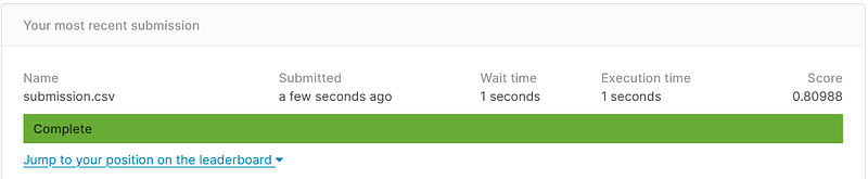
It was roughly six hours of high intensity work from the time a topic was decided on and we presented. Shortly after things finished, we made a late submission to see how we did and placed near the 60th percentile with a multi-class loss of 0.80988, which isn’t bad for how rushed and quick we did things.

The longer you work on something, it is harder and harder to squeeze more out of things. It’s not uncommon, where there is a limit or asymptote to the results you can achieve. It was very much a case when I was writing my thesis and reminds me of the mathematicians ordering beer. If we had cut the loss by 0.1 (12%), we would’ve been in the top 99.5%. We can continue to cut the distance between where we are and 0, but the closer we are the harder it is to push that little bit further. I can order a beer, then half of one, then half of that, and so on just to end up with two beers. I could go back and try to squeeze more out of our fit, but in the 6 hours of work we were able to accomplish so much, and I am proud of mine and my teams work.
